TS Imagine Historical VaR (HVaR) has become a standard measurement of risk, in which a current portfolio is subjected to the market conditions of a prior day and the resulting P&L is recorded. This experiment is repeated over many different days from the past, and the resulting outcomes are aggregated into a P&L probability distribution in which any day from the past is equally probable of reoccurring.
This approach is considered to be more realistic than earlier tools that simply assumed that returns were normally distributed; no such assumption is required for HVaR – it just is what it is.
The two most important features of HVaR, and the reasons why it has become so broadly accepted are:
- There is no mystery in how it is computed. Everyone agrees on the calculation, and it comes down to having the requisite history of returns available.
- Extreme historical events are more likely to be included, that would be otherwise excluded by an assumption of normality. These are the so-called “fat tails.”
However, in practice there is a very large wrinkle that is usually regarded as an inconvenience to be either ignored or dealt with in a perfunctory manner – herein lies the core issue. The Lookback Period (“Window”).
When computing HVaR, one must first decide upon which historical dates to use. These are usually specified by a “window” of dates, stretching back several years. This window has typically been around three years. However that is now changing.
Many firms now require a full twelve years of prices (plus data from further back such as the Great Recession of 2008 – 2009). However, this requirement introduces a conundrum: what do we do when a company has not been around for the full window? In fact, fully half of today’s US equities are less than twelve years old. Prominent examples include Facebook (META), Tesla and Alibaba.
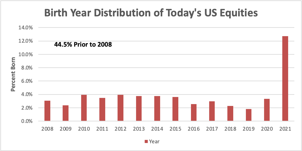
This table displays the distribution by birth year, going back to 2008.
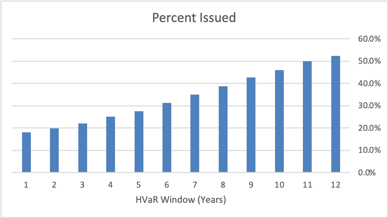
We can also recast this information in terms of the HVaR window: For a given lookback period of HVaR, what percent of the US equities were first issued during that window?
So now a decision has to be made as to how to deal with those stocks that were “born” during the window. This means that we are already diverging from point 1; different firms may make different choices. So let’s try to make the best choices we can.
First Option: (ignore)
Treat the newborns as having zero returns for the dates prior to the birthdate.
The Problem:
Keep in mind that the purpose of HVaR is to assess today’s risk. This assumption will underestimate the risk due to the new stocks, and therefore the HVaR. Many of today’s S&P stocks were not even listed twelve years ago including Facebook (META), Tesla and Alibaba.
Second Option: (most common)
Estimate each stock’s beta against a benchmark index (typically the S&P500 for US Stocks) and proxy the returns using the returns on the index.
The Problem:
This introduces some unintended consequences: the returns that are being fabricated will be perfectly correlated with each other, and more importantly the synthetic returns will not adequately capture the tail risk. In fact, this second option is guaranteed to miss the tails; it’s an inherent deficiency in the approach. The following example explains why.
Example: Proxying returns using a single factor.
Let’s write the returns in the usual way as:
![]() with uncorrelated. Then (ignoring the mean),
with uncorrelated. Then (ignoring the mean),
![]()
So that in particular the standard deviation is ![]()
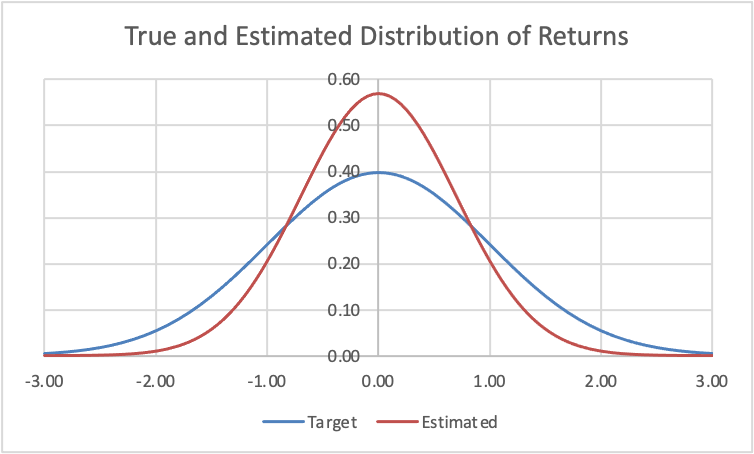
In fact, in terms of R squared(R-squared), we have . In practice, ordinary regression will yield an R squared in the 0.2 – 0.7 range, so that in any case the standard deviation of the proxy returns are at least 30% less than those of the actual returns. Now suppose for the moment that both sets of returns are normally distributed. Then as the following graph makes clear, the proxy return distribution simply cannot properly capture the tail behavior. But that’s where HVaR lives. And so if this approach can’t even work for the case of normal returns, there is no hope for it in the real world.
Third Option: (tail weighted factors)
A better solution is to determine, if you can, a weighted multifactor representation of the missing returns. This approach goes like this:
- Determine a set of factors that collectively best approximate the returns of the target stock
- The factors themselves need to have the full twelve years+ of history
- Regress the factor returns against the target returns over whatever period is available to determine the weights (a.k.a. multivariate betas).
- However, perform a weighted regression that places more emphasis on the returns with a higher magnitude
Note: The collection of factors can be tailored to each target stock. There is no requirement to use the same factors across the entire portfolio. This freedom enables us to achieve the best fit possible.
The details of this approach are rather technical, and so will be further explored in a white paper (Coming soon: Predicting the Past – Enriching the HVaR Calculation).
However, we can illustrate the effect by a simple comparison.
Example: 1.0% HVaR for a long portfolio of ten equally weighted equities, all born in 2018, calculated for various windows.
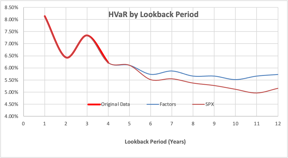
This graph shows that when the data is falling back, the weighted factor HVaR does a much better job at maintaining the tails that contribute to HVaR. (For the initial 4 year lookback period in all three cases the actual data is being used, so that the graphs coincide in that region.)
Conclusion
The calculation of HVaR will almost always require some proxying of returns. This often overlooked issue can materially affect the outcome of the HVaR simulations, and so should be thought through very carefully. Fortunately, there are robust solutions available that preserve the essential fat tail nature of the resulting distribution of returns.